57. The Income Fluctuation Problem I: Basic Model #

In addition to what’s in Anaconda, this lecture will need the following libraries:

!pip install quantecon

57.1. Overview #

In this lecture, we study an optimal savings problem for an infinitely lived consumer—the “common ancestor” described in [Ljungqvist and Sargent, 2018], section 1.3.

This is an essential sub-problem for many representative macroeconomic models

It is related to the decision problem in the cake eating model and yet differs in important ways.

For example, the choice problem for the agent includes an additive income term that leads to an occasionally binding constraint.

Moreover, shocks affecting the budget constraint are correlated, forcing us to track an extra state variable.

To solve the model we will use the endogenous grid method, which we found to be fast and accurate in our investigation of cake eating.

We’ll need the following imports:

import matplotlib.pyplot as plt
import numpy as np
from quantecon import MarkovChain
import jax
import jax.numpy as jnp
from typing import NamedTuple

57.1.1. References#

We skip most technical details but they can be found in [Ma et al., 2020].

Other references include [Deaton, 1991], [Den Haan, 2010], [Kuhn, 2013], [Rabault, 2002], [Reiter, 2009] and [Schechtman and Escudero, 1977].

57.2. The Optimal Savings Problem #

Let’s write down the model and then discuss how to solve it.

57.2.1. Set-Up#

Consider a household that chooses a state-contingent consumption plan \(\{c_t\}_{t \geq 0}\) to maximize

\[ \mathbb{E} \, \sum_{t=0}^{\infty} \beta^t u(c_t) \]

subject to

(57.1)#\[a_{t+1} + c_t \leq R a_t + Y_t \quad c_t \geq 0, \quad a_t \geq 0 \quad t = 0, 1, \ldots\]

Here

\(\beta \in (0,1)\) is the discount factor
\(a_t\) is asset holdings at time \(t\), with borrowing constraint \(a_t \geq 0\)
\(c_t\) is consumption
\(Y_t\) is non-capital income (wages, unemployment compensation, etc.)
\(R := 1 + r\), where \(r > 0\) is the interest rate on savings

The timing here is as follows:

At the start of period \(t\), the household observes labor income \(Y_t\) and financial assets \(R a_t\) .
The household chooses current consumption \(c_t\).
Time shifts to \(t+1\) and the process repeats.

Non-capital income \(Y_t\) is given by \(Y_t = y(Z_t)\), where

\(\{Z_t\}\) is an exogenous state process and
\(y\) is a given function taking values in \(\mathbb{R}_+\).

As is common in the literature, we take \(\{Z_t\}\) to be a finite state Markov chain taking values in \(\mathsf Z\) with Markov matrix \(\Pi\).

We further assume that

\(\beta R < 1\)
\(u\) is smooth, strictly increasing and strictly concave with \(\lim_{c \to 0} u'(c) = \infty\) and \(\lim_{c \to \infty} u'(c) = 0\)
\(y(z) = \exp(z)\)

The asset space is \(\mathbb R_+\) and the state is the pair \((a,z) \in \mathsf S := \mathbb R_+ \times \mathsf Z\).

A feasible consumption path from \((a,z) \in \mathsf S\) is a consumption sequence \(\{c_t\}\) such that \(\{c_t\}\) and its induced asset path \(\{a_t\}\) satisfy

\((a_0, z_0) = (a, z)\)
the feasibility constraints in (57.1), and
measurability, which means that \(c_t\) is a function of random outcomes up to date \(t\) but not after.

The meaning of the third point is just that consumption at time \(t\) cannot be a function of outcomes are yet to be observed.

In fact, for this problem, consumption can be chosen optimally by taking it to be contingent only on the current state.

Optimality is defined below.

57.2.2. Value Function and Euler Equation#

The value function \(V \colon \mathsf S \to \mathbb{R}\) is defined by

(57.2)#\[V(a, z) := \max \, \mathbb{E} \left\{ \sum_{t=0}^{\infty} \beta^t u(c_t) \right\}\]

where the maximization is overall feasible consumption paths from \((a,z)\).

An optimal consumption path from \((a,z)\) is a feasible consumption path from \((a,z)\) that attains the supremum in (57.2).

To pin down such paths we can use a version of the Euler equation, which in the present setting is

(57.3)#\[ u' (c_t) \geq \beta R \, \mathbb{E}_t u'(c_{t+1})\]

and

(57.4)#\[ c_t < a_t \; \implies \; u' (c_t) = \beta R \, \mathbb{E}_t u'(c_{t+1})\]

When \(c_t = a_t\) we obviously have \(u'(c_t) = u'(a_t)\),

When \(c_t\) hits the upper bound \(a_t\), the strict inequality \(u' (c_t) > \beta R \, \mathbb{E}_t u'(c_{t+1})\) can occur because \(c_t\) cannot increase sufficiently to attain equality.

(The lower boundary case \(c_t = 0\) never arises at the optimum because \(u'(0) = \infty\).)

57.2.3. Optimality Results#

As shown in [Ma et al., 2020],

For each \((a,z) \in \mathsf S\), a unique optimal consumption path from \((a,z)\) exists
This path is the unique feasible path from \((a,z)\) satisfying the Euler equations (57.3)-(57.4) and the transversality condition

(57.5)#\[\lim_{t \to \infty} \beta^t \, \mathbb{E} \, [ u'(c_t) a_{t+1} ] = 0\]

Moreover, there exists an optimal consumption policy \(\sigma^* \colon \mathsf S \to \mathbb R_+\) such that the path from \((a,z)\) generated by

\[ (a_0, z_0) = (a, z), \quad c_t = \sigma^*(a_t, Z_t) \quad \text{and} \quad a_{t+1} = R (a_t - c_t) + Y_{t+1} \]

satisfies both the Euler equations (57.3)-(57.4) and (57.5), and hence is the unique optimal path from \((a,z)\).

Thus, to solve the optimization problem, we need to compute the policy \(\sigma^*\).

57.3. Computation #

We solve for the optimal consumption policy using time iteration and the endogenous grid method.

Readers unfamiliar with the endogenous grid method should review the discussion in Cake Eating V: The Endogenous Grid Method.

57.3.1. Solution Method#

We rewrite (57.4) to make it a statement about functions rather than random variables:

(57.6)#\[ (u' \circ \sigma) (a, z) = \beta R \, \sum_{z'} (u' \circ \sigma) [R a + y(z) - \sigma(a, z)), \, z'] \Pi(z, z')\]

Here

\((u' \circ \sigma)(s) := u'(\sigma(s))\),
primes indicate next period states (as well as derivatives), and
\(\sigma\) is the unknown function.

We aim to find a fixed point \(\sigma\) of (57.6).

To do so we use the EGM.

We begin with an exogenous grid \(G = \{a'_0, \ldots, a'_{m-1}\}\) with \(a'_0 = 0\).

Fix a current guess of the policy function \(\sigma\).

For each \(a'_i\) and \(z_j\) we set

\[ c_{ij} = (u')^{-1} \left[ \beta R \, \sum_{z'} u' [ \sigma(a'_i, z') ] \Pi(z_j, z') \right] \]

and then \(a^e_{ij}\) as the current asset level \(a_t\) that solves the budget constraint \(a'_{ij} + c_{ij} = R a_t + y(z_j)\).

That is,

\[ a^e_{ij} = \frac{1}{R} [a'_{ij} + c_{ij} - y(z_j)]. \]

Our next guess policy function, which we write as \(K\sigma\), is the linear interpolation of \((a^e_{ij}, c_{ij})\) over \(i\), for each \(j\).

(The number of one dimensional linear interpolations is equal to len(z_grid).)

For \(a < a^e_{ij}\) we use the budget constraint to set \((K \sigma)(a, z_j) = Ra + y(z_j)\).

57.4. Implementation #

We use the CRRA utility specification

\[ u(c) = \frac{c^{1 - \gamma}} {1 - \gamma} \]

57.4.1. Set Up#

Here we build a class called IFP that stores the model primitives.

class IFP(NamedTuple):
    R: float                  # Gross interest rate R = 1 + r
    β: float                  # Discount factor
    γ: float                  # Preference parameter
    Π: jnp.ndarray            # Markov matrix for exogenous shock
    z_grid: jnp.ndarray       # Markov state values for Z_t
    asset_grid: jnp.ndarray   # Exogenous asset grid


def create_ifp(r=0.01,
               β=0.98,
               γ=1.5,
               Π=((0.6, 0.4),
                  (0.05, 0.95)),
               z_grid=(0.0, 0.2),
               asset_grid_max=40,
               asset_grid_size=50):

    asset_grid = jnp.linspace(0, asset_grid_max, asset_grid_size)
    Π, z_grid = jnp.array(Π), jnp.array(z_grid)
    R = 1 + r
    assert R * β < 1, "Stability condition violated."
    return IFP(R=R, β=β, γ=γ, Π=Π, z_grid=z_grid, asset_grid=asset_grid)

# Set y(z) = exp(z)
y = jnp.exp

The exogenous state process \(\{Z_t\}\) defaults to a two-state Markov chain with transition matrix \(\Pi\).

We define utility globally:

# Define utility function derivatives
u_prime = lambda c, γ: c**(-γ)
u_prime_inv = lambda c, γ: c**(-1/γ)

57.4.2. Solver#

Here is the operator \(K\) that transforms current guess \(\sigma\) into next period guess \(K\sigma\).

We understand \(\sigma\) is an array of shape \((n_a, n_z)\), where \(n_a\) and \(n_z\) are the respective grid sizes.

The value σ[i,j] corresponds to \(\sigma(a'_i, z_j)\).

def K(σ: jnp.ndarray, ifp: IFP) -> jnp.ndarray:
    """
    The Coleman-Reffett operator for the IFP model using the
    Endogenous Grid Method.

    This operator implements one iteration of the EGM algorithm to
    update the consumption policy function.

    Algorithm
    ---------
    The EGM works backwards from next period:
    1. Given σ(a', z'), compute current consumption c that
       satisfies Euler equation
    2. Compute the endogenous current asset level a^e that leads
       to (c, a')
    3. Interpolate back to exogenous grid to get σ_new(a', z')

    """
    R, β, γ, Π, z_grid, asset_grid = ifp
    n_a = len(asset_grid)
    n_z = len(z_grid)

    def compute_c_for_fixed_income_state(j):
        """
        Compute updated consumption policy for income state z_j.

        The asset_grid here represents a' (next period assets).

        """

        # Compute u'(σ(a', z')) for all (a', z')
        u_prime_vals = u_prime(σ, γ)

        # Calculate the sum Σ_{z'} u'(σ(a', z')) * Π(z_j, z') at each a'
        expected_marginal = u_prime_vals @ Π[j, :]

        # Use Euler equation to find today's consumption
        c_vals = u_prime_inv(β * R * expected_marginal, γ)

        # Compute endogenous grid of current assets using the 
        a_endogenous = (1/R) * (asset_grid + c_vals - y(z_grid[j]))

        # Interpolate back to exogenous grid
        σ_new = jnp.interp(asset_grid, a_endogenous, c_vals)

        # For asset levels below the minimum endogenous grid point,
        # the household is constrained and c = R*a + y(z) 

        σ_new = jnp.where(asset_grid < a_endogenous[0],
                          R * asset_grid + y(z_grid[j]),
                          σ_new)

        return σ_new  #  Consumption over the asset grid given z[j]

    # Compute consumption over all income states using vmap
    c_vmap = jax.vmap(compute_c_for_fixed_income_state)
    σ_new = c_vmap(jnp.arange(n_z)) # Shape (n_z, n_a), one row per income state

    return σ_new.T  # Transpose to get (n_a, n_z) 

@jax.jit
def solve_model(ifp: IFP,
                σ_init: jnp.ndarray,
                tol: float = 1e-5,
                max_iter: int = 1000) -> jnp.ndarray:
    """
    Solve the model using time iteration with EGM.

    """

    def condition(loop_state):
        i, σ, error = loop_state
        return (error > tol) & (i < max_iter)

    def body(loop_state):
        i, σ, error = loop_state
        σ_new = K(σ, ifp)
        error = jnp.max(jnp.abs(σ_new - σ))
        return i + 1, σ_new, error

    initial_state = (0, σ_init, tol + 1)
    final_loop_state = jax.lax.while_loop(condition, body, initial_state)
    i, σ, error = final_loop_state

    return σ

57.4.3. Test run#

Let’s road test the EGM code.

ifp = create_ifp()
R, β, γ, Π, z_grid, asset_grid = ifp
σ_init = R * asset_grid[:, None] + y(z_grid)
σ_star = solve_model(ifp, σ_init)

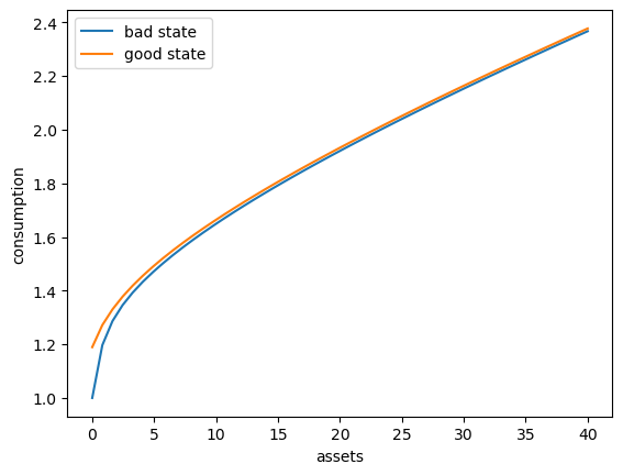
Here’s a plot of the optimal policy for each \(z\) state

fig, ax = plt.subplots()
ax.plot(asset_grid, σ_star[:, 0], label='bad state')
ax.plot(asset_grid, σ_star[:, 1], label='good state')
ax.set(xlabel='assets', ylabel='consumption')
ax.legend()
plt.show()

_images/f44b1684246c6b303f94159f42e5d5098d5fc03962269095a0d0a125f00b7c8b.png

To begin to understand the long run asset levels held by households under the default parameters, let’s look at the 45 degree diagram showing the law of motion for assets under the optimal consumption policy.

ifp = create_ifp()
R, β, γ, Π, z_grid, asset_grid = ifp
σ_init = R * asset_grid[:, None] + y(z_grid)
σ_star = solve_model(ifp, σ_init)
a = asset_grid

fig, ax = plt.subplots()
for z, lb in zip((0, 1), ('low income', 'high income')):
    ax.plot(a, R * (a - σ_star[:, z]) + y(z) , label=lb)

ax.plot(a, a, 'k--')
ax.set(xlabel='current assets', ylabel='next period assets')

ax.legend()
plt.show()

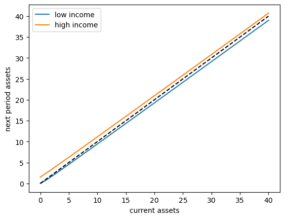
_images/05caf7a048bb856b2ec3a4118047eb4af686168c173d8656377952dec824373a.png

The unbroken lines show the update function for assets at each \(z\), which is

\[ a \mapsto R (a - \sigma^*(a, z)) + y(z) \]

The dashed line is the 45 degree line.

The figure suggests that the dynamics will be stable — assets do not diverge even in the highest state.

In fact there is a unique stationary distribution of assets that we can calculate by simulation – we examine this below.

Can be proved via theorem 2 of [Hopenhayn and Prescott, 1992].
It represents the long run dispersion of assets across households when households have idiosyncratic shocks.

57.4.4. A Sanity Check#

One way to check our results is to

set labor income to zero in each state and
set the gross interest rate \(R\) to unity.

In this case, our income fluctuation problem is just a CRRA cake eating problem.

Then the value function and optimal consumption policy are given by

def c_star(x, β, γ):
    return (1 - β ** (1/γ)) * x


def v_star(x, β, γ):
    return (1 - β**(1 / γ))**(-γ) * (x**(1-γ) / (1-γ))

Let’s see if we match up:

ifp_cake_eating = create_ifp(r=0.0, z_grid=(-jnp.inf, -jnp.inf))
R, β, γ, Π, z_grid, asset_grid = ifp_cake_eating
σ_init = R * asset_grid[:, None] + y(z_grid)
σ_star = solve_model(ifp_cake_eating, σ_init)

fig, ax = plt.subplots()
ax.plot(asset_grid, σ_star[:, 0], label='numerical')
ax.plot(asset_grid,
        c_star(asset_grid, ifp_cake_eating.β, ifp_cake_eating.γ),
        '--', label='analytical')
ax.set(xlabel='assets', ylabel='consumption')
ax.legend()
plt.show()

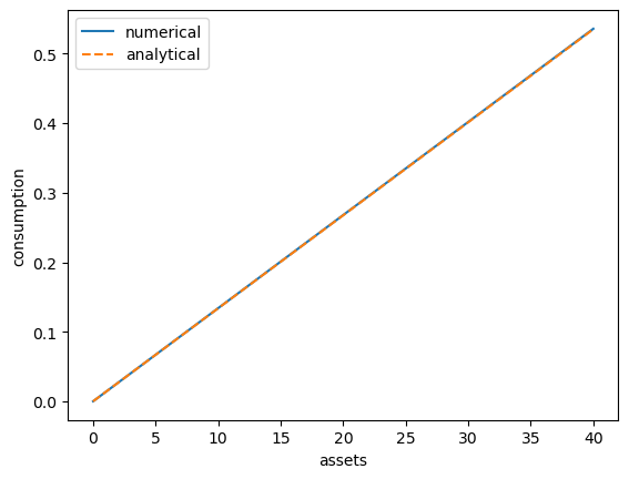
_images/b67dd0260a63f9b6947d935b70431b0f33606bd526ab790867964bb5abd79e47.png

This looks pretty good.

57.5. Exercises #

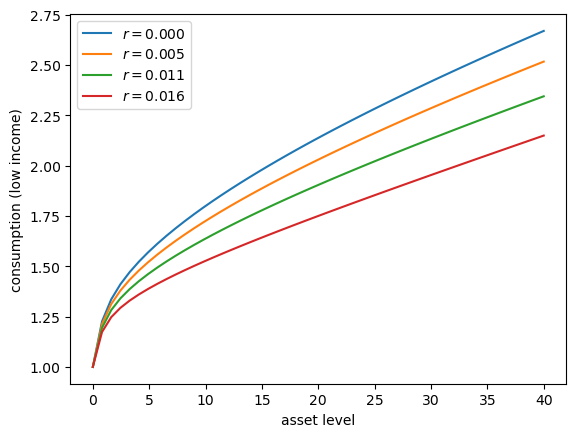
Exercise 57.1

Let’s consider how the interest rate affects consumption.

Step r through np.linspace(0, 0.016, 4).
Other than r, hold all parameters at their default values.
Plot consumption against assets for income shock fixed at the smallest value.

Your figure should show that, for this model, higher interest rates boost suppress consumption (because they encourage more savings).

Solution

Here’s one solution:

# With β=0.98, we need R*β < 1, so r < 0.0204
r_vals = np.linspace(0, 0.016, 4)

fig, ax = plt.subplots()
for r_val in r_vals:
    ifp = create_ifp(r=r_val)
    R, β, γ, Π, z_grid, asset_grid = ifp
    σ_init = R * asset_grid[:, None] + y(z_grid)
    σ_star = solve_model(ifp, σ_init)
    ax.plot(asset_grid, σ_star[:, 0], label=f'$r = {r_val:.3f}$')

ax.set(xlabel='asset level', ylabel='consumption (low income)')
ax.legend()
plt.show()

_images/80951cfb296fd93863dfd89b7a9af027909e33dc5f68db89280add6c8c5616e5.png

Exercise 57.2

Let’s approximate the stationary distribution by simulation.

Run a large number of households forward for \(T\) periods and then histogram the cross-sectional distribution of assets.

Set num_households=50_000, T=500.

Solution

First we write a function to simulate many households in parallel using JAX.

def compute_asset_stationary(ifp, σ_star, num_households=50_000, T=500, seed=1234):
    """
    Simulates num_households households for T periods to approximate
    the stationary distribution of assets.

    By ergodicity, simulating many households for moderate time is equivalent
    to simulating one household for very long time, but parallelizes better.

    ifp is an instance of IFP
    σ_star is the optimal consumption policy
    """
    R, β, γ, Π, z_grid, asset_grid = ifp
    n_z = len(z_grid)

    # Create interpolation function for consumption policy
    σ_interp = lambda a, z_idx: jnp.interp(a, asset_grid, σ_star[:, z_idx])

    # Simulate one household forward
    def simulate_one_household(key):
        # Random initial state (both z and a)
        key1, key2, key3 = jax.random.split(key, 3)
        z_idx = jax.random.choice(key1, n_z)
        # Start with random assets drawn uniformly from [0, asset_grid_max/2]
        a = jax.random.uniform(key3, minval=0.0, maxval=asset_grid[-1]/2)

        # Simulate forward T periods
        def step(state, key_t):
            a_current, z_current = state
            # Draw next shock
            z_next = jax.random.choice(key_t, n_z, p=Π[z_current])
            # Update assets
            z_val = z_grid[z_next]
            c = σ_interp(a_current, z_next)
            a_next = R * a_current + y(z_val) - c
            return (a_next, z_next), None

        keys = jax.random.split(key2, T)
        (a_final, _), _ = jax.lax.scan(step, (a, z_idx), keys)
        return a_final

    # Vectorize over many households
    key = jax.random.PRNGKey(seed)
    keys = jax.random.split(key, num_households)
    assets = jax.vmap(simulate_one_household)(keys)

    return np.array(assets)

Now we call the function, generate the asset distribution and histogram it:

ifp = create_ifp()
R, β, γ, Π, z_grid, asset_grid = ifp
σ_init = R * asset_grid[:, None] + y(z_grid)
σ_star = solve_model(ifp, σ_init)
assets = compute_asset_stationary(ifp, σ_star)

fig, ax = plt.subplots()
ax.hist(assets, bins=20, alpha=0.5, density=True)
ax.set(xlabel='assets')
plt.show()

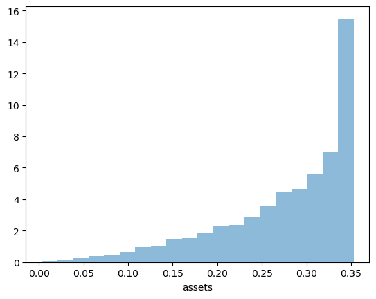
_images/f7be94e900fa281fa57d145d29389213d53fd7051642aea5e081f82044bcc7b4.png

The shape of the asset distribution is unrealistic.

Here it is left skewed when in reality it has a long right tail.

In a subsequent lecture we will rectify this by adding more realistic features to the model.

Exercise 57.3

Following on from exercises 1 and 2, let’s look at how savings and aggregate asset holdings vary with the interest rate

Note

[Ljungqvist and Sargent, 2018] section 18.6 can be consulted for more background on the topic treated in this exercise.

For a given parameterization of the model, the mean of the stationary distribution of assets can be interpreted as aggregate capital in an economy with a unit mass of ex-ante identical households facing idiosyncratic shocks.

Your task is to investigate how this measure of aggregate capital varies with the interest rate.

Following tradition, put the price (i.e., interest rate) on the vertical axis.

On the horizontal axis put aggregate capital, computed as the mean of the stationary distribution given the interest rate.

Solution

Here’s one solution

M = 25
# With β=0.98, we need R*β < 1, so R < 1/0.98 ≈ 1.0204, thus r < 0.0204
r_vals = np.linspace(0, 0.015, M)
fig, ax = plt.subplots()

asset_mean = []
for r in r_vals:
    print(f'Solving model at r = {r}')
    ifp = create_ifp(r=r)
    R, β, γ, Π, z_grid, asset_grid = ifp
    σ_init = R * asset_grid[:, None] + y(z_grid)
    σ_star = solve_model(ifp, σ_init)
    assets = compute_asset_stationary(ifp, σ_star, num_households=10_000, T=500)
    mean = np.mean(assets)
    asset_mean.append(mean)
    print(f'  Mean assets: {mean:.4f}')
ax.plot(r_vals, asset_mean)

ax.set(xlabel='interest rate', ylabel='capital')

plt.show()

Solving model at r = 0.0

  Mean assets: 0.0000
Solving model at r = 0.000625

  Mean assets: 0.0000
Solving model at r = 0.00125

  Mean assets: 0.0000
Solving model at r = 0.001875

  Mean assets: 0.0000
Solving model at r = 0.0025

  Mean assets: 0.0000
Solving model at r = 0.003125

  Mean assets: 0.0085
Solving model at r = 0.00375

  Mean assets: 0.0293
Solving model at r = 0.004375

  Mean assets: 0.0507
Solving model at r = 0.005

  Mean assets: 0.0728
Solving model at r = 0.005625

  Mean assets: 0.0955
Solving model at r = 0.00625

  Mean assets: 0.1189
Solving model at r = 0.006875

  Mean assets: 0.1430
Solving model at r = 0.0075

  Mean assets: 0.1679
Solving model at r = 0.008125

  Mean assets: 0.1936
Solving model at r = 0.00875

  Mean assets: 0.2202
Solving model at r = 0.009375

  Mean assets: 0.2477
Solving model at r = 0.01

  Mean assets: 0.2762
Solving model at r = 0.010625

  Mean assets: 0.3057
Solving model at r = 0.01125

  Mean assets: 0.3364
Solving model at r = 0.011875

  Mean assets: 0.3683
Solving model at r = 0.0125

  Mean assets: 0.4014
Solving model at r = 0.013125

  Mean assets: 0.4359
Solving model at r = 0.01375

  Mean assets: 0.4720
Solving model at r = 0.014375

  Mean assets: 0.5096
Solving model at r = 0.015

  Mean assets: 0.5490

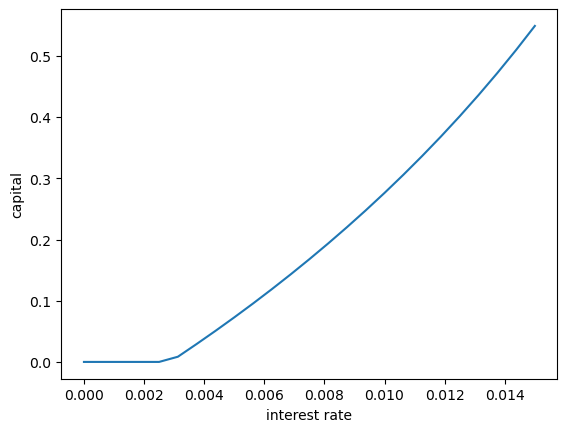
_images/413dcc6ca19815e5d0f4d6554fbc89100edf51f9da6b3986c31599bf47de160f.png

As expected, aggregate savings increases with the interest rate.

57. The Income Fluctuation Problem I: Basic Model#

57.1. Overview#

57.1.1. References#

57.2. The Optimal Savings Problem#

57.2.1. Set-Up#

57.2.2. Value Function and Euler Equation#

57.2.3. Optimality Results#

57.3. Computation#

57.3.1. Solution Method#

57.4. Implementation#

57.4.1. Set Up#

57.4.2. Solver#

57.4.3. Test run#

57.4.4. A Sanity Check#

57.5. Exercises#

57. The Income Fluctuation Problem I: Basic Model #

57.1. Overview #

57.2. The Optimal Savings Problem #

57.3. Computation #

57.4. Implementation #

57.5. Exercises #